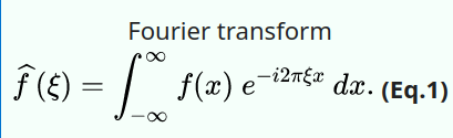
# An intuitive grasp over Fourier Transform
I have a lot of things in my life I've always wanted to understand but for some reason the maths were too hard for me. One of my good old nemesis was the Fourier Transform
I am not that good at mathematical abstractions so in order to understand something I prefer to take the opposite path and then see the reason of it. Why is it useful? Why all the fuss?
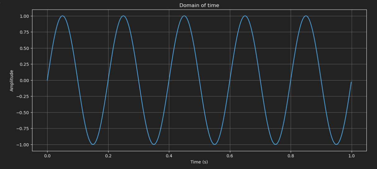
A Fourier transform is a way to decompose a signal into its components. If we have a signal with frequency of 5Hz and another with 50Hz combined I will have something like
import numpy as np
import matplotlib.pyplot as plt
from scipy.fftpack import fft, fftfreq

def signal(t):
    return np.sin(2 * np.pi * 5 * t) + 0.5 * np.sin(2 * np.pi * 50 * t)

sampling_rate = 1000
T = 1.0 / sampling_rate
t = np.arange(0, 1.0, T)
y = signal(t)

Y = fft(y)
N = len(t)
freqs = fftfreq(N, T)
Let's draw this signal
plt.figure(figsize=(14, 6))
plt.plot(t, y)
plt.title('Domain of time')
plt.xlabel('Time (s)')
plt.ylabel('Amplitude')
plt.grid()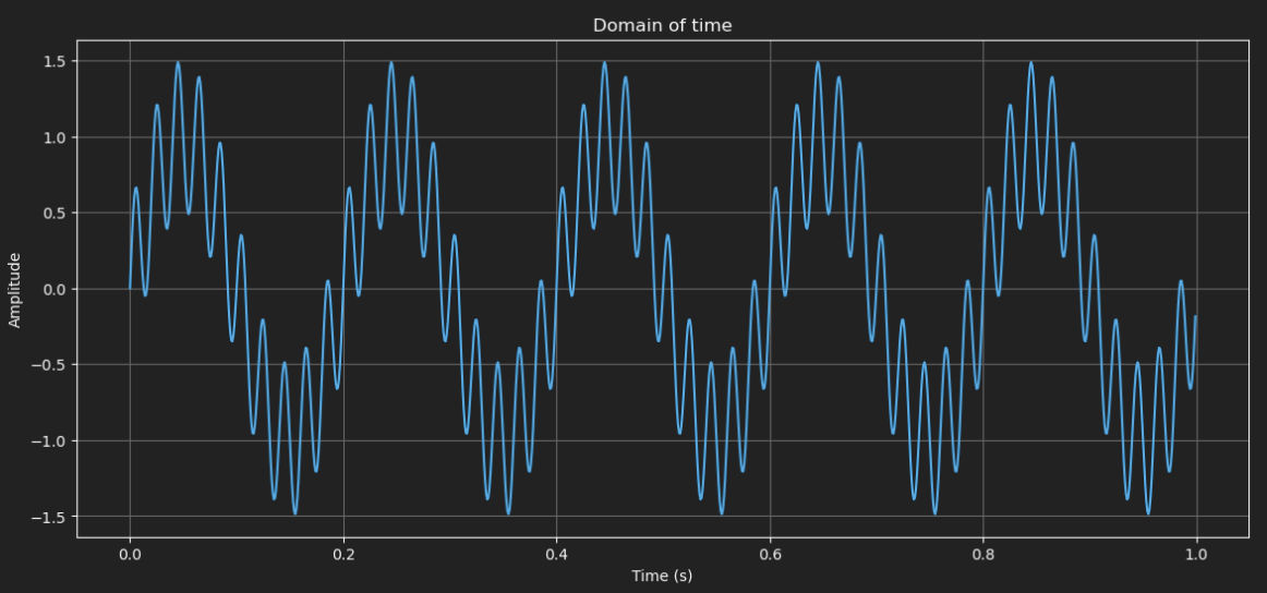
You can see the big wave to be the 5Hz signal and the much faster wave the 50Hz signal.
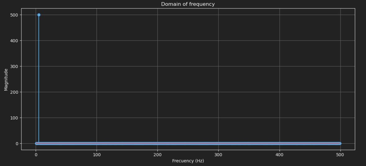
If I apply Fourier transform to that and plot the absolute value of the result I will have something like.
plt.figure(figsize=(14, 6))
plt.plot(freqs[freqs>0], np.abs(Y)[freqs>0])
plt.title('Domain of frequency')
plt.xlabel('Frecuency (Hz)')
plt.ylabel('Magnitude')
plt.grid()

plt.show()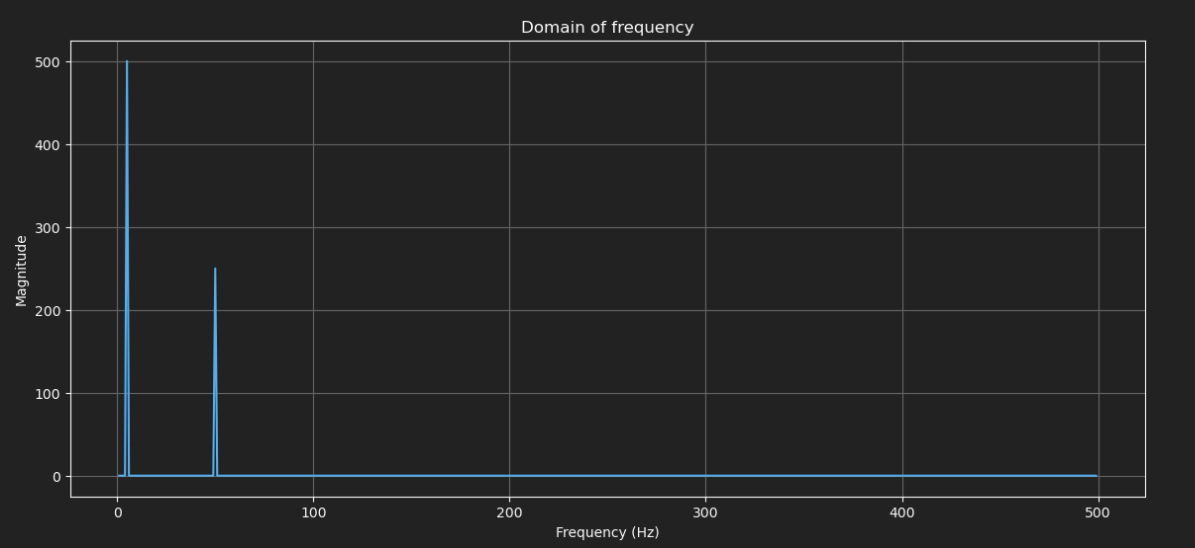
There are two peaks. One at 5 and another at 50. If we draw with stems it will be more clear
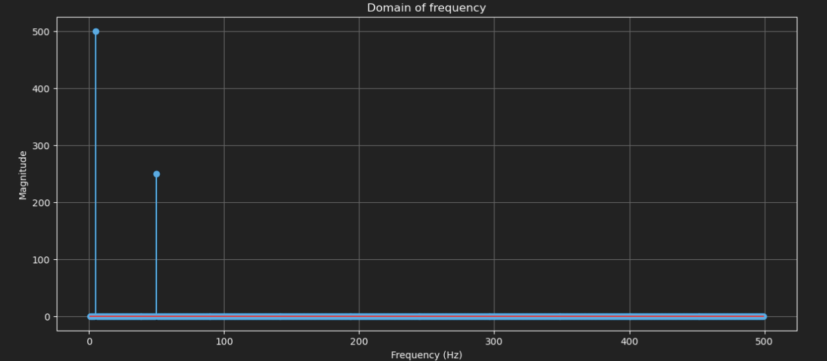
Exactly the ones we generated the wave from. But... still... why is this useful?
There are two things that I didn't explain yet:
- We can also do this for sampled signals, not only for continuous ones
- This is a two way transform
Let's start with the former. I can do Fourier transform on, for example a wav file. A wav file are sound wave samples at a given frequency (normally 44000 or 48000 Hz) and decompose them. We can do the same with color waves in an image or even whatever we think can behave as a signal. That makes the potential applications endless.
This being a two way transform is the final piece of the puzzle. I can go back and forth from Fourier transform to original signal. This allows us to manipulate components of the signal with ease and get back to the original.
In our previous example let's imagine that we consider the 50Hz signal (the one that vibrates more) to be noise. Let's do a small noise gate and filter that signal in the frequency domain
Y_filtered = Y.copy()
Y_filtered[50] = 0
Y_filtered[-50] = 0
This filtered signal will show as
So if we do the inverse Fourier over it
from scipy.fftpack import ifft

filtered_y = ifft(Y_filtered)
We get
We did something that can be improved, though, in the lines
Y_filtered[50] = 0
Y_filtered[-50] = 0
In out code we have that array called freqs. Since the array indexes are discrete values and a signal is a continuum we have this kind of arrays so we can know what the indexes are. In reality that 50 we want to filter is not an exact point but we have do do a small range. Let's say we want to do 0.1 wide.
Y_filtered[np.abs(freqs - 50) < 0.1] = 0
Y_filtered[np.abs(freqs + 50) < 0.1] = 0
That will set to zero all values that are at less than 0.1 to the 50Hz point. From 49999 to 50001. Probably we will have just one in our array but depending on the resolution you may have more.
So now we should have some super basic intuition about how this works, why is important and how we can use it.
Happy hacking!